Biogas From Waste Example

Background Information

In the Biogas From Waste example, cattle farms produce manure which is then processed by a technology site, which uses anaerobic digestion to produce biogas and digestate (a waste product). The biogas is then purchased by customers or further processed by another technology site to produce electricity, and the digestate is applied to a crop field.

Since there are many cattle farms, technology sites, and consumers, there are many combinations of pathways that the manure and biogas can take. We would like to find out which pathway is the most economically favorable.

We only want to manage sites that already exist; we are not considering building new technology sites. This type of problem can be defined as a management-type model.

Outline

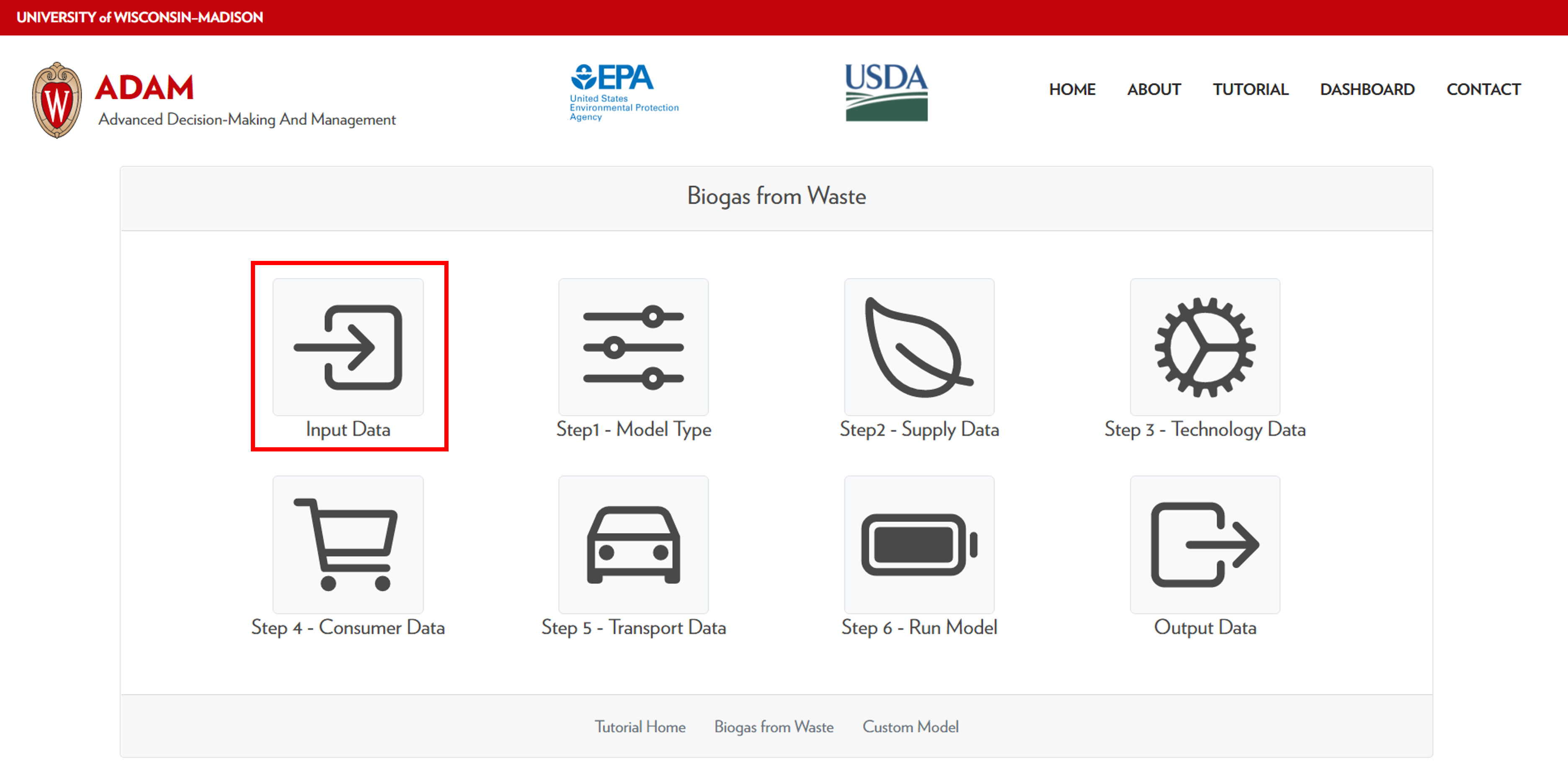
The first screen you encounter is the Outline Page. This page provides an overview of the steps we will go over during the tutorial. You may select any of the icons to jump to that part of the tutorial. For first-time users, we recommend selecting the Input Data step.

Input Data

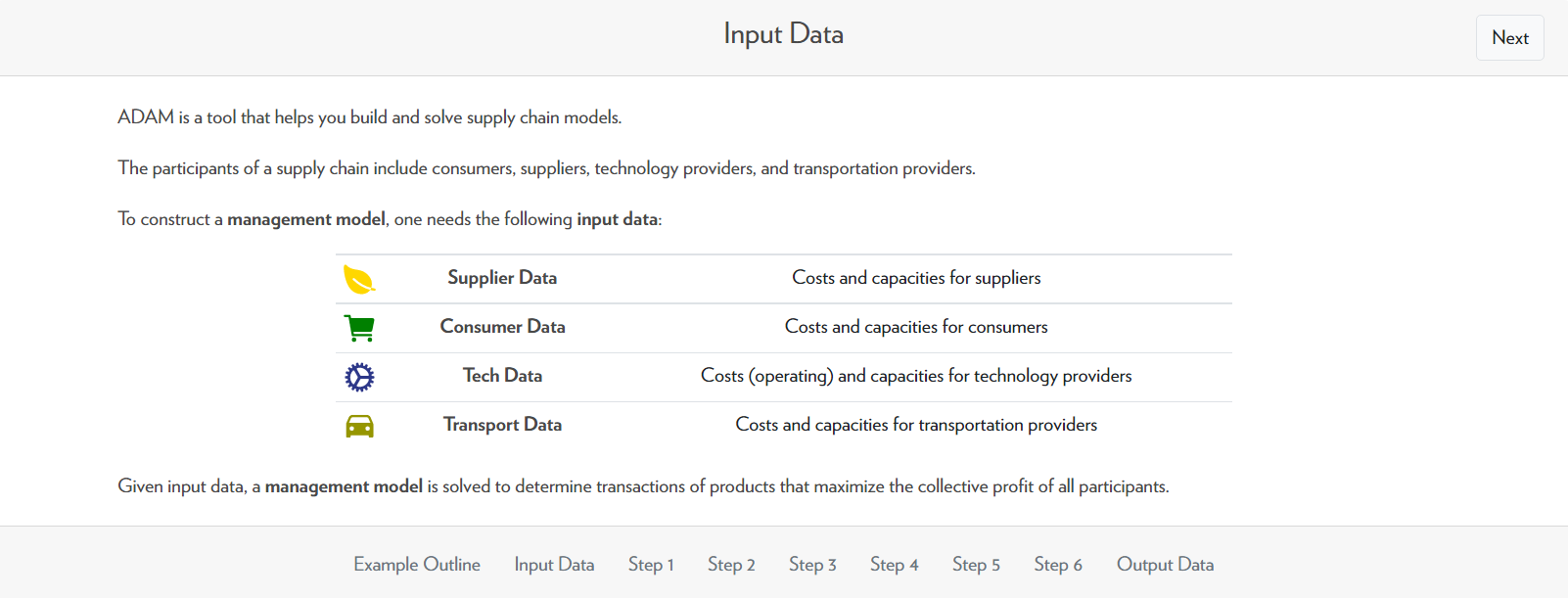
The first page of the tutorial gives you information about the input data needed for ADAM. This input data consists of supply data, demand data, technology data, and transportation data.

The Supplier Data

In the case of biogas to waste, the suppliers are CAFOs that produce cattle manure. The supplier data includes several pieces of information about each CAFO: their location, the amount of manure produced (capacity), and the cost of the waste to the supplier.

The Consumer Data

The consumers are any person or organization that purchases a valuable product. Similar to the supplier data, the consumer data includes the following information about each consumer: their location, the maximum amount of product they can purchase (capacity), and the unit price at which they are buying the product. In this case, the only product of value is the biogas produced by the technology sites.

The Technology Data

Technologies are any equipment, factory, or process that can transform one product into another. In the context of biogas from waste, the technology being used is an anaerobic digester that uses cattle manure to produce biogas (main product) and digestate (a waste product). The technology data includes the location and type of technology installed.

The Transportation Data

The transportation data includes information on the transportation costs of each product based on distance traveled. ADAM automatically generates this data.

Step 1 - Model Type

Now that we have gone over the input data for this example, we can now select the model-type and time basis. As stated before, since we are only focusing on managing existing technologies, we select a management-type model rather than a design-type model (the custom model demonstrates the design type-model).

The time basis is set to Year. For future steps, you will have to make sure that the units are consistent with the time basis selected.

Step 2 - Supply Data

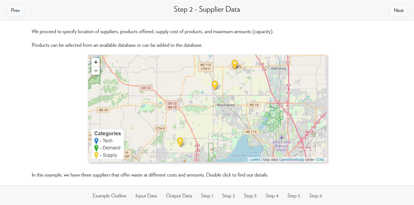
After defining the model type and time basis, we can now add supplier data. In this example, there are three suppliers which are indicated by the yellow markers on the map.

By double-clicking on any of the markers, you can get more detailed information about each node. An example of the detailed information is shown below.

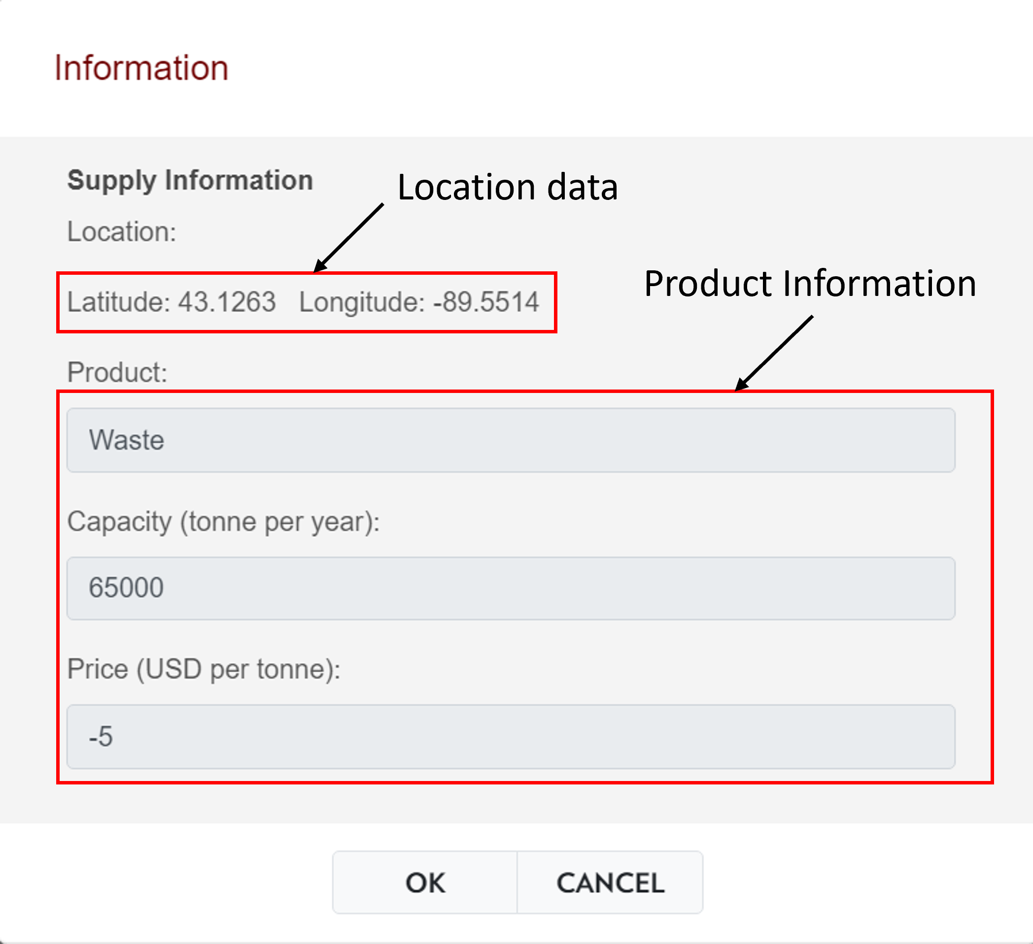
Here we see that this supply node is located at a longitude and latitude of 43.1263, -89.5514. It produces waste at a capacity of 65,000 tonnes per year (the “per year” was defined in step 1) at a cost of $5 per tonne of waste produced.

A negative price indicates a reverse money flow (i.e. the supplier loses money while the consumer gains money). This is true for a waste management system because waste is an undesireable product, therefore the suppliers have to pay money in order to get rid of it.

Step 3 - Consumer Data

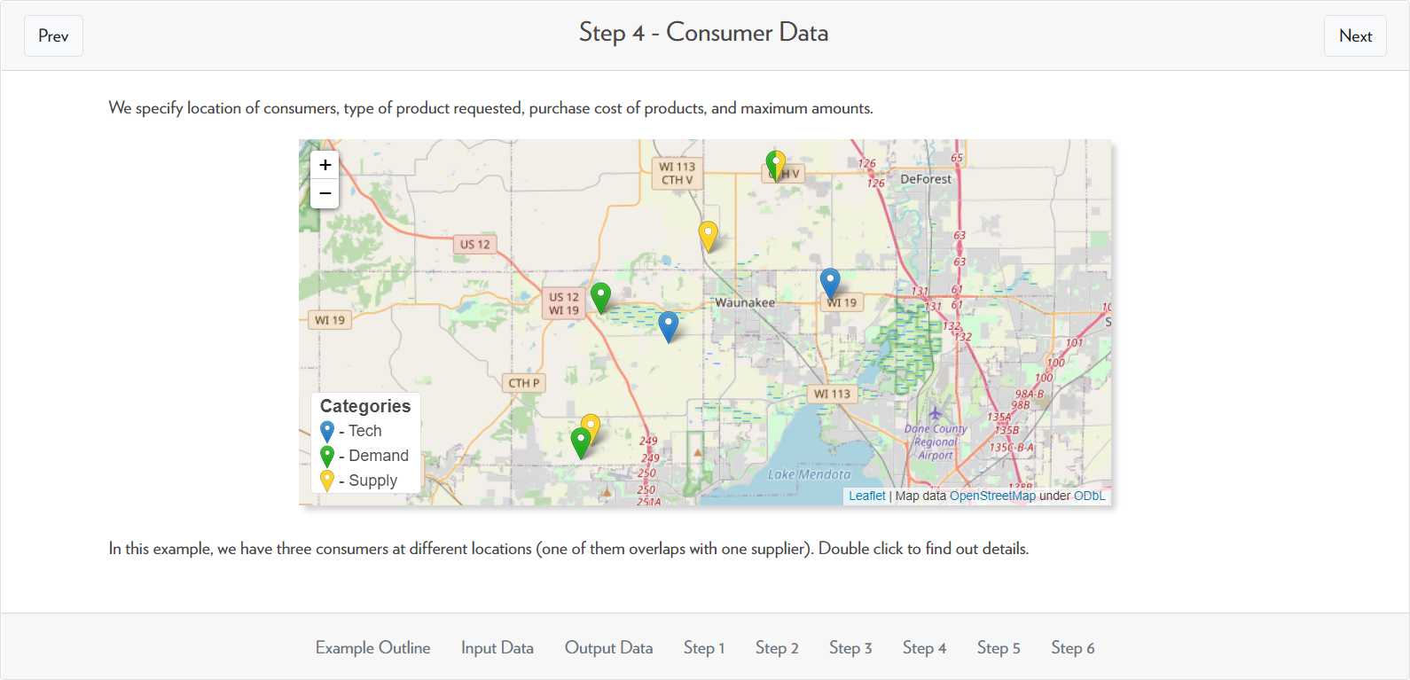
In step 3, we define the consumer (demand) data. In this example, we have three demand data nodes indicated on the map as green markers. Note that the topmost node is both a supply and a demand node, indicated by a half-green and half-yellow marker. This is not exclusive to supply and demand information. A single node can act as a supply, demand, and technology node or any combination of the three.

Double-clicking on the demand node will open more detailed information about that node. An example of this is shown below:

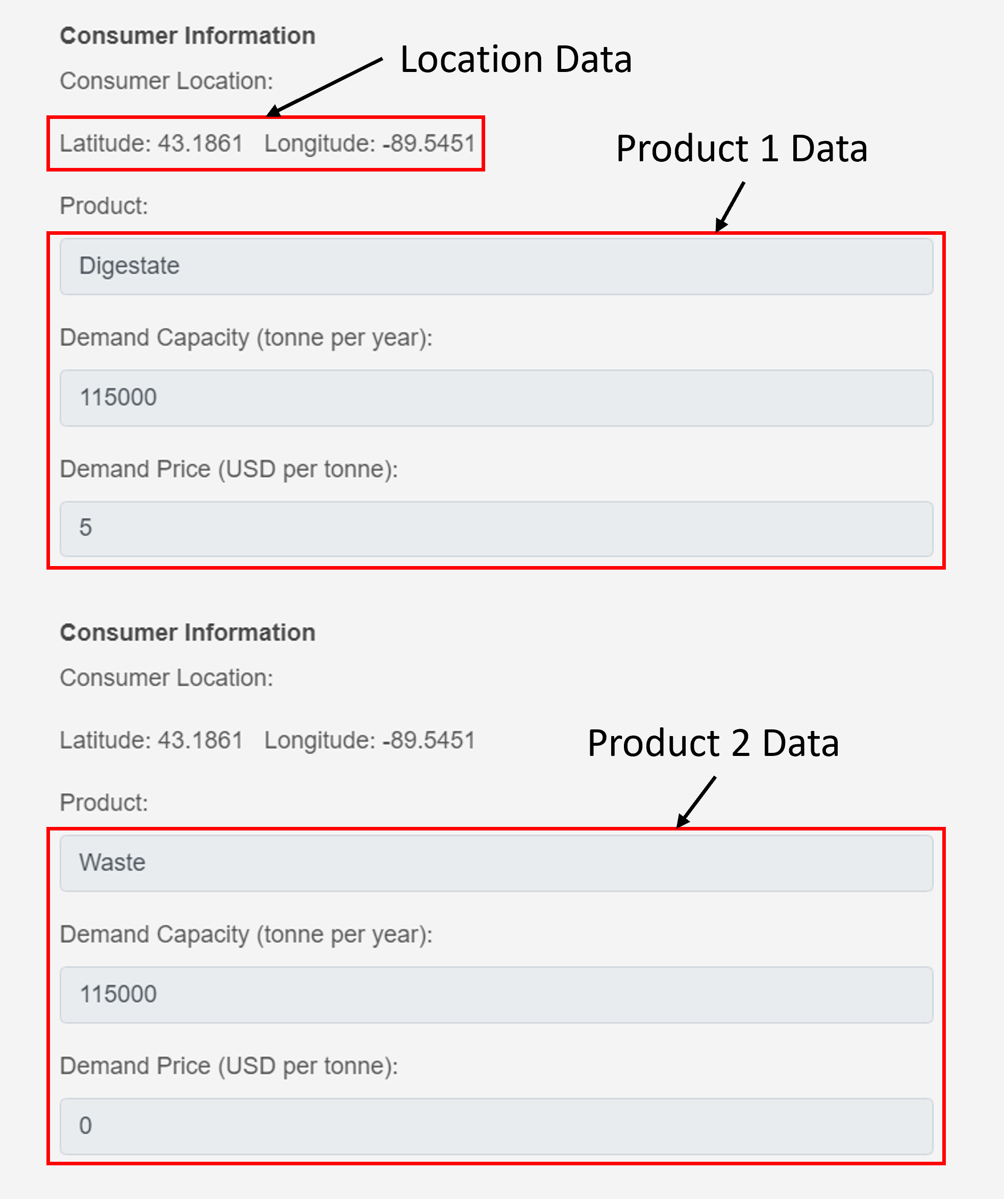
This consumer demands two different products: digestate and waste. Digestate is the waste product of the technology after it processes waste into biogas. The consumer demands 115,000 tonnes per year of both digestate and waste. They purchase the digestate for $5 per tonne, and they get the waste at no cost. The consumer can get the waste at zero cost because the supplier loses money by producing waste so the supplier would like to get rid of the waste while sustaining as little losses as possible.

This consumer only wants the waste products, meaning that this consumer is likely a crop field that demands the nutrients from the manure.

Step 4 - Technology Data

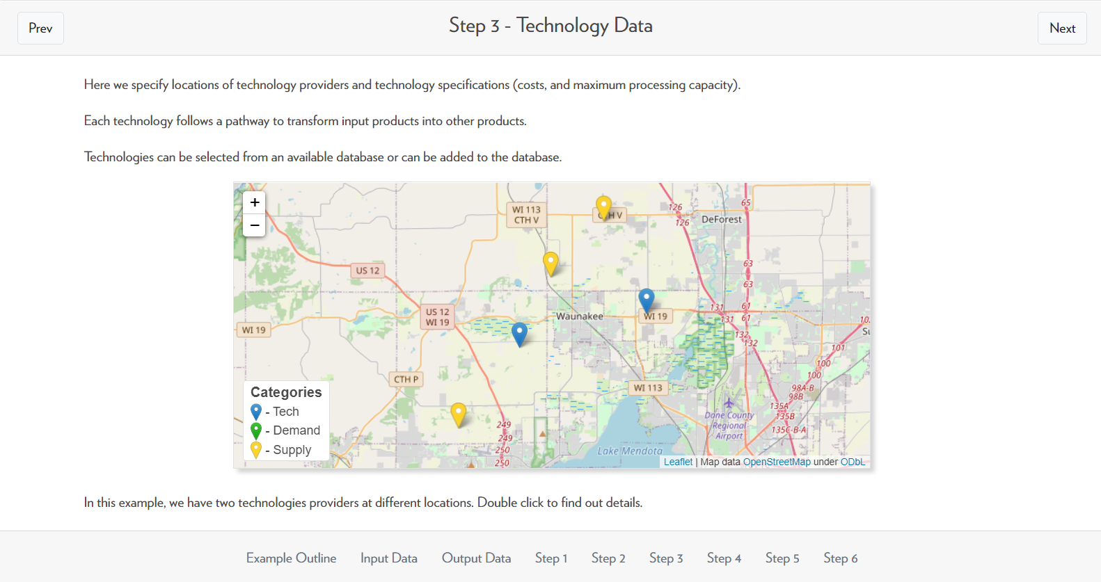
In step 4, we define the technology nodes. In this example, we have two technology nodes which are shown on the map as the blue markers.

Similar to the supply nodes, double-clicking on the technology nodes will give you more information about that node. An example of the detailed information is shown below.

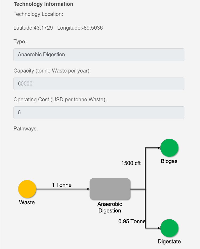
From this detailed information, we can determine that this is an anaerobic digestion type technology located at a longitude and latitude of 43.1729, -89.5036. It can process up to 60,000 tonnes of waste per year (again the “per year” was defined in step 1) at a cost of $6 per tonne of waste processed.

The diagram at the bottom of the detailed information window shows the inputs and outputs of the technology. For every 1 tonne of waste, the anaerobic digestion technology produces 1500 cubic ft of biogas and 0.95 tonnes of digestate.

Step 5 - Transport Data

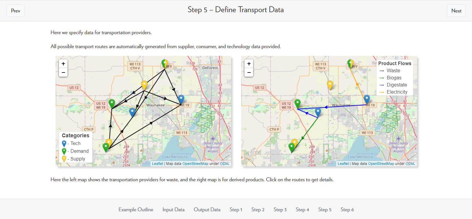
After defining all of the supply, demand, and technology nodes, we can now define transportation data. The graph on the left shows all possible transportation routes for waste and the graph on the right shows all transportation routes for every other product.

Hovering over the route until the white information box appears, then clicking on the route will display additional information.

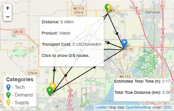
This route is between the markers labeled CAFO2 and Technology2. The distance between the markers is 6.49 km, the product being transported is waste, and the waste is being transported at $3 per tonne per km. The box in the lower right corner shows that the “true” distance (i.e. the distance it would take to drive from one point to the other using roads) is 8.56 km. It also gives a time estimate based on an average car’s speed.

Step 6 - Run Model

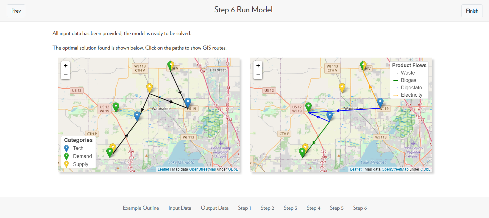
The final step is running the model using ADAM to find the optimal routes that each of the products should take. Hovering over and clicking on the routes will show the amount of product flow and the transportation cost that will allow each member of the system to have maximum benefits.

In this case, it appears that it is most favorable for each of the supply nodes to send a portion of their waste to be processed at a technology site. One of the technology sites produces digestate and biogas, and the other produces digestate and electricity. Consumer1 buys the biogas, Consumer2 buys the digestate, and Consumer3 buys the electricity.

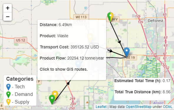
Looking at the same pathway as before, there is now information about the amount of waste transported (product flow). In this case, waste is being transported across this pathway at a rate of 20,294.12 tonnes/year with a transportation cost of $395,126.52.

Output Data

After we give ADAM all of the input data, ADAM will generate output data which includes information about the flow, transportation, and value data.

The flow data shows the amount of product transported along each pathway (e.g. 10,000 tonnes/year), the transportation data shows the transportation cost of moving the product from one place to another, and the value data shows the value of the products at different locations.