Custom Model Example

Background information

In a custom model, you can define the supply, demand, and technology data to specify the problem you want to solve. For this example, we will be exploring a different type of model: a design-type model. Rather than simply managing technology sites that already exist, a design-type model will decide whether to build a technology at a certain site. Additionally, it will calculate the performance of the system, including the technologies that were worth building.

Outline

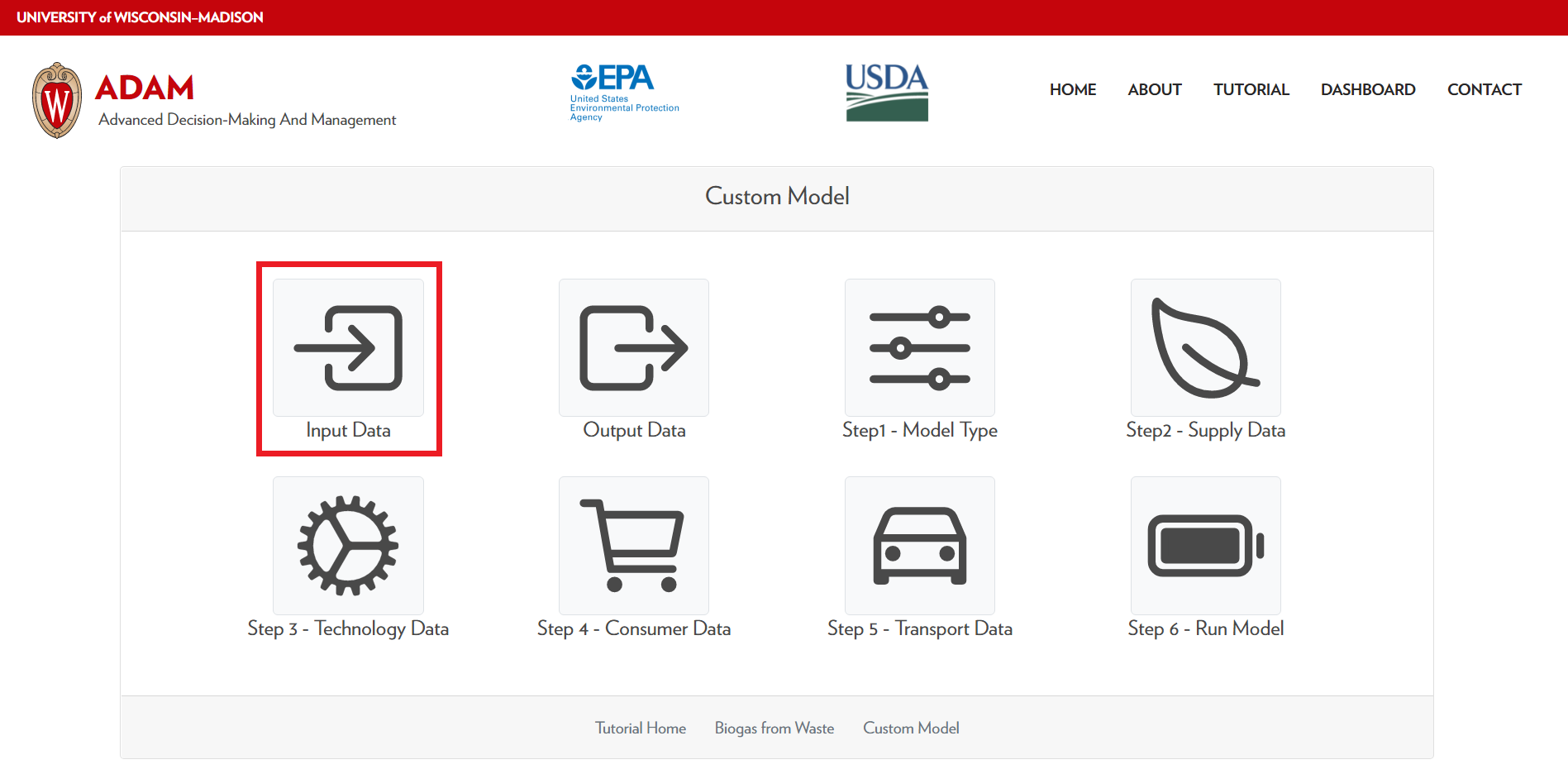
The first screen you encounter is the Outline Page. This page provides an overview of the steps we will go over during the tutorial. We reccomend going through the tutorial in order. Do this by selecting the Input Data step.

Input Data

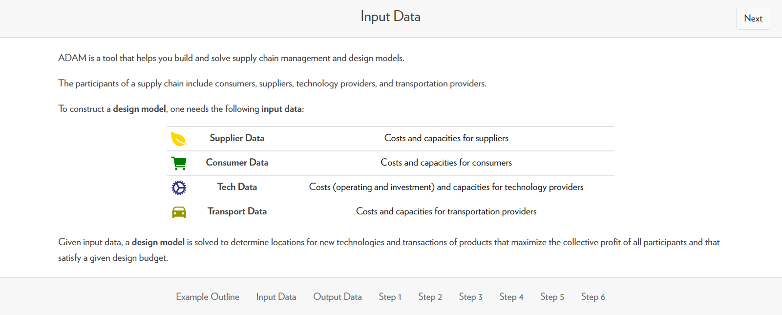
Similar to the biogas from waste example, the inputs for the custom model are supply data, customer data, technology data, and transportation data. The only difference is the information included in the technology data.

In the biogas from waste example, the technology data only included information about existing technology sites; however, for a design-type model, we must also consider technology candidates, sites where technologies could potentially be built.

All other inputs are the same as the biogas from waste example except the suppliers and customers are generic; the suppliers do not need to be CAFOs and the consumers do not need to be the same as the ones in the biogas from waste example.

Output Data

The outputs of the custom model include flow data, transportation data, value data, and design data.

The flow data shows the amount of product transported along each pathway, the transportation data shows the transportation cost of moving the product from one place to another, the value data shows the value of the products at different locations, and the design data shows the technologies that should be installed at each location.

Step 1 - Model Type

For the first step of creating a model, we must define the model-type and time basis. As stated before, this example will go over a design-type model. The time-basis is left as year which is the default setting.

Step 2 - Supply Data

The supply data of a custom model can be anything that supplies a product (usually a waste product). In this example three CAFOs acting as supply nodes are provided; you can click and drag the nodes or edit the data as you wish.

We can edit the capacity and price of the points. Remember that capacity refers to the amount of product that the supply node produces, and the price refers to the cost of the product to the supplier.

The video below shows the capacity of CAFO1 being changed from 65,000 to 50,000 tonnes of manure per year; the price is changed from costing the CAFO $5 per tonne to $10 per tonne. Remember that a negative price indicates cost.

Step 3 - Comsumer Data

The consumers in this model are any person, place, or thing that demands a product and are indicated by the green nodes. You can click and drag the nodes to different locations.

Similar to the other steps we have encountered, you can also double-click the nodes to edit the demand information about each consumer. In the video below, Consumer4's capacity is changed from 30,000 to 60,000 gallons of biomethane per year, and its price is changed from $3,000 to $3,500 per gallon. This means that Consumer4 now demands a maximum of 60,000 gallons of biomethane per year and is willing to buy the biomethane at $3,500 per gallon.

Step 4 - Technology Data

The technology data includes technology sites, which are locations that have pre-existing technologies, and technology candidates, which are locations where a technology could be built.

In this example, there are two technology sites (blue) and one technology candidate (red). You can click and drag these points to different locations.

You can also double-click to edit the capacities of the technology sites. The technology candidate node cannot be edited. In the video below, Technology1's capacity is changed from 60,000 to 80,000 tonnes of waste. This means that Technology1 can now process 20,000 more tonnes of waste than it could before.

Step 5 - Transportation Data

The transportation data gives information on the product that is being transported, the transportation cost, and the distance that the product is transported.

You can hover over each transportation route to see detailed information and click to see the estimated time and the distance for that pathway. The "true distance" refers to the distance that the vehicle travels in order to get from one point to another. "Distance" simply refers to the distance between one point to another if you were to travel in a straight line.

The video below demonstrates how to display the pathway details on the left and right graphs. It can be a bit tricky to find out exactly where to hover over the route to display the information.

Step 6 - Run Model

After you have completed steps 1 through 5, you will have the option to run the model. Using the data that you have provided, ADAM will then find the optimal routes that the products will take, and it will determine whether or not the technology should be installed at the technology candidate location.

Running the model may take a few minutes. Please do not refresh or exit out of the page while it is running.

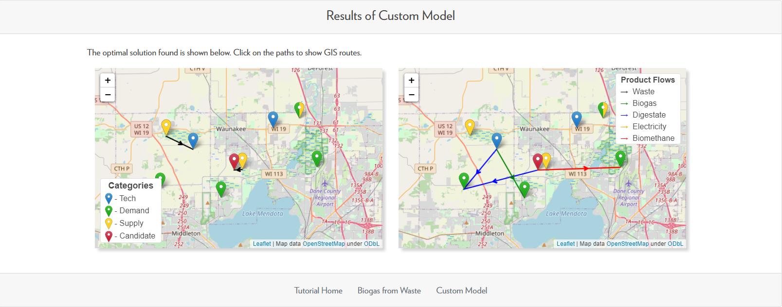
An example of the results is shown below. The left graph shows that two out of the three CAFOs should send their waste to a technology site. Since there is a pathway going to the technology candidate node, this means that building the technology and processing waste there is worth doing.

The right graph shows the product pathways from the technology sites to the consumers. Hovering over the pathways would quantitatively show the amount of product that is being transported across that pathway and the total transportation cost of moving that amount of product.

Try going through the custom model tutorial on your own to get familiar with ADAM!